More advanced example
From CrewWiki
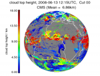
Display a cloud property of one algorithm on the MSG disk
o=obj_new('cws_stats')

o->set_product,'cth'

o->set_group,'CMS'

o->set_date,2008,6,13,12,15

o->make_image, /single

obj_destroy, o
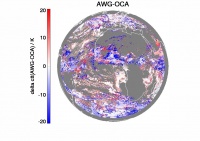
Difference of one data set to another (one picture per algorithm pair)
o=obj_new('cws_stats')

o->set_product,'ctt'

o->set_date,2008,6,13,12,00

o->diff_maps, group='AWG'

obj_destroy, o
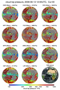
Display a cloud property of all algorithms on the MSG disk
o=obj_new('cws_stats')

o->set_product,'ctp'

o->set_date,2008,6,13,12,00

o->make_image, /no_track

obj_destroy, o
Calculate multi algorithm ensemble average
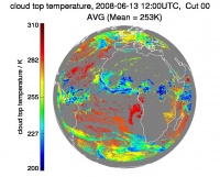
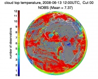
Note, first you have to calculate the multi ensemble average with o->algorithm_average(/calc, /save, mask='com'). As the default resolution is a reduced resolution, you have to specify explecitely the scale=1, when you create the cws_stats object. If the average file is created, you can handle the average like a group by setting the group to 'AVG' and make plots like in the other examples (and of cause you can use the default reduced resolution again). By setting the group to 'NOBS' you can make plots of the number of algorithm observation.
o=obj_new('cws_stats', scale=1)

o->set_product,'ctt'

o->set_date,2008,6,13,12,00

avg = o->algorithm_average(/calc, /save, mask='com')

o->set_group,'AVG'

o->make_image, /single

o->set_group,'NOBS'

o->make_image, /single

obj_destroy, o
Calculate multi algorithm ensemble standard deviation
Note, first you have to calculate (and save) the multi algorithm ensemble average like in the example before. Then you have to calculate the multi algorithm ensemble standard deviation. Like in the example before, you have to specify explecitely the scale=1, when you create the cws_stats object. If the standard deviation file is created, you can handle the absolute and relative standard deviations like a group by setting the group to 'STD_ABS' and 'STD_REL' respectively, and make plots like in the other examples (and of cause you can use the default reduced resolution again).
o=obj_new('cws_stats', scale=1)

o->set_product,'ctt'

o->set_date,2008,6,13,12,00

std_abs = o->algorithm_stddev (/calc, /save, mask='com')

o->set_group,'STD_ABS'

o->make_image, /single, min=0, max=20

std_rel = o->algorithm_stddev (/calc, /save, mask='com', /relative)

o->set_group,'STD_REL'

o->make_image, /single

obj_destroy, o


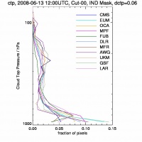
1d histogram
o=obj_new('cws_stats')

o->set_product,'ctp'

o->set_date,2008,6,13,12,00

o->hist1d

obj_destroy, o
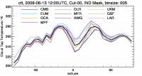
dependency on latitude
o=obj_new('cws_stats')

o->set_product,'cth'

o->set_date,2008,6,13,12,00

o->dep

obj_destroy, o
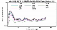
dependency on viewing zenith angle
o=obj_new('cws_stats')

o->set_product,'ctp'

o->set_date,2008,6,13,12,00

o->dep, /vza

obj_destroy, o
Simple statistics as a table
o=obj_new('cws_stats')

o->set_product,'ctp'

o->set_date,2008,6,13,12,00

o->make_tables

obj_destroy, o

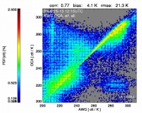
Two algorithm scatter plot
o=obj_new('cws_stats')

o->set_product,'ctt'

o->set_date,2008,6,13,12,00

o->make_corSingle

obj_destroy, o
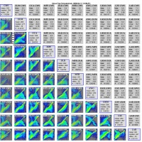
Thumbnails of all scatter plots
o=obj_new('cws_stats')

o->set_product,'ctt'

o->set_date,2008,6,13,12,00

o->make_corThumb

obj_destroy, o
